Stay home and plot Density of States

This is a tutorial on plotting total and partial Density of States for electronic structure calculations performed with the DFT code VASP.

Being a computational condensed matter physicist who spends most of his day on a computer, one might think that COVID-19¹ may not have made drastic changes to my work routine. In theory, this is a valid argument since I should be able to work from anywhere as long as I have a network connection that allows me to connect to our supercomputing clusters. However, I tend to be more productive at work since there are less distractions that sway me out of focus. So I made some changes at home which included moving my TV and PS4 to the living room and finding timeworthy hobbies to keep myself occupied. Dedicating time for my website is one of them. So I will try to post more frequently from now on.

Plotting Density of States

The density of states (DOS) of a material gives a measure of the number of energy states available in the system that electrons are allowed to occupy. DOS is an essential quantity to predict a material’s conductivity. I won’t be diving into the derivations but there’s plenty of resources on the internet that cover that.²

VASP is one of the main DFT³ codes I use for electronic structure calculations. Although there are excellent methods to plot DOS such as p4vasp⁴, being a GUI application it becomes quite inefficient when we have to deal with data from hundreds of calculations. This is where command line applications fare better.

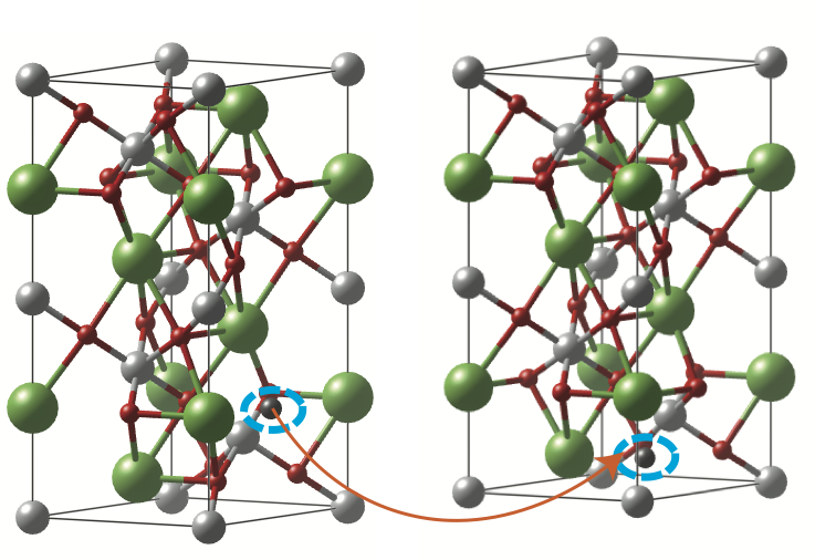
I recently performed DFT calculations for hundreds of different oxygen vacancy configurations of rare-earth Nickelates in an attempt to study the effect of these vacancies on the conductivity of the material. Plotting DOS was part of the plan. So I wrote a script based on the great pymatgen⁵ to do exactly that.

For this tutorial we will plot the DOS of the paramagnetic metal LaNiO\(_3\). Its crystal structure is displayed below.

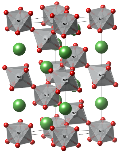
La, Ni and O are represented with green, gray and red, respectively. In terms of a POSCAR format that would look like:

 La Ni O| SG: R-3c 167 PG: -3m BL: R | sym_eps: 0.019194 (WICKOFF R-3c #167)
 1.000000
    5.41650000000000   0.00000000000000   0.00000000000000
   -2.70825000000000   4.69082659959841   0.00000000000000
    0.00000000000000   0.00000000000000  12.92470000000000
 6 6 18
 Direct
    0.00000000000000   0.00000000000000   0.25000000000000  La
    0.00000000000000   0.00000000000000   0.75000000000000  La
    0.66666666666667   0.33333333333333   0.58333333333333  La
    0.66666666666667   0.33333333333333   0.08333333333333  La
    0.33333333333333   0.66666666666667   0.91666666666667  La
    0.33333333333333   0.66666666666667   0.41666666666667  La
    0.00000000000000   0.00000000000000   0.00000000000000  Ni
    0.00000000000000   0.00000000000000   0.50000000000000  Ni
    0.66666666666667   0.33333333333333   0.33333333333333  Ni
    0.66666666666667   0.33333333333333   0.83333333333333  Ni
    0.33333333333333   0.66666666666667   0.66666666666667  Ni
    0.33333333333333   0.66666666666667   0.16666666666667  Ni
    0.44805661000000   0.00000000000000   0.25000000000000  O
    0.00000000000000   0.44805661000000   0.25000000000000  O
		...
    0.78138994333333   0.11472327666667   0.41666666666667  O

The script we will use is called plotDOS.py and can be found in this repository. The following command will give you a list of options when run from the calculation directory.

plotDOS.py -h

Total DOS

This is the total contribuition from all the atoms and orbitals in the system.

Run:

plotDOS.py total -show

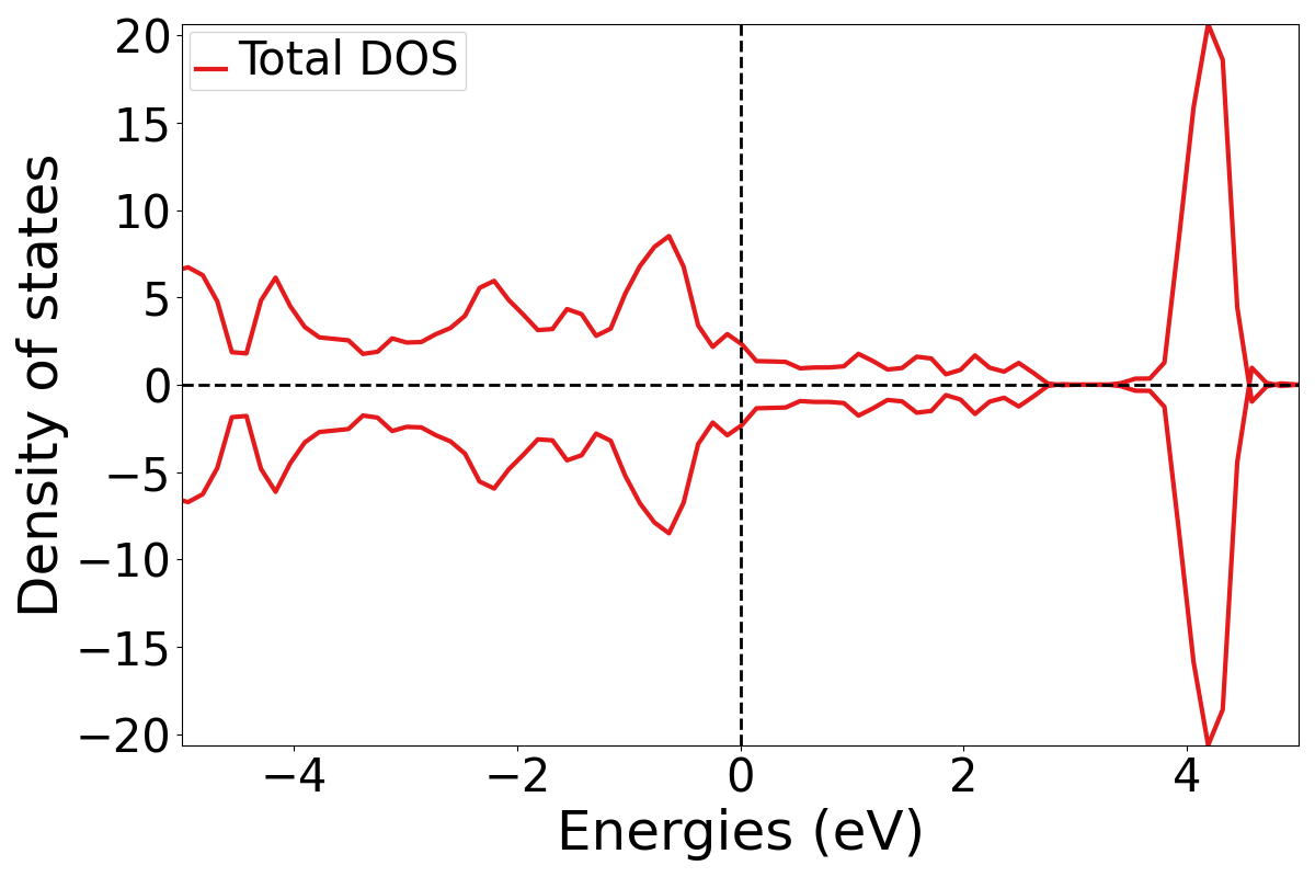
The -show flag displays the plot on screen. Otherwise it would just save the figure as a .png file. As you can see since there are states at the Fermi level this is classified as a metal. The total DOS is rather boring so let’s move on to plotting partial DOS where we can see the different contributions of atoms and orbitals to the DOS.

Partial DOS

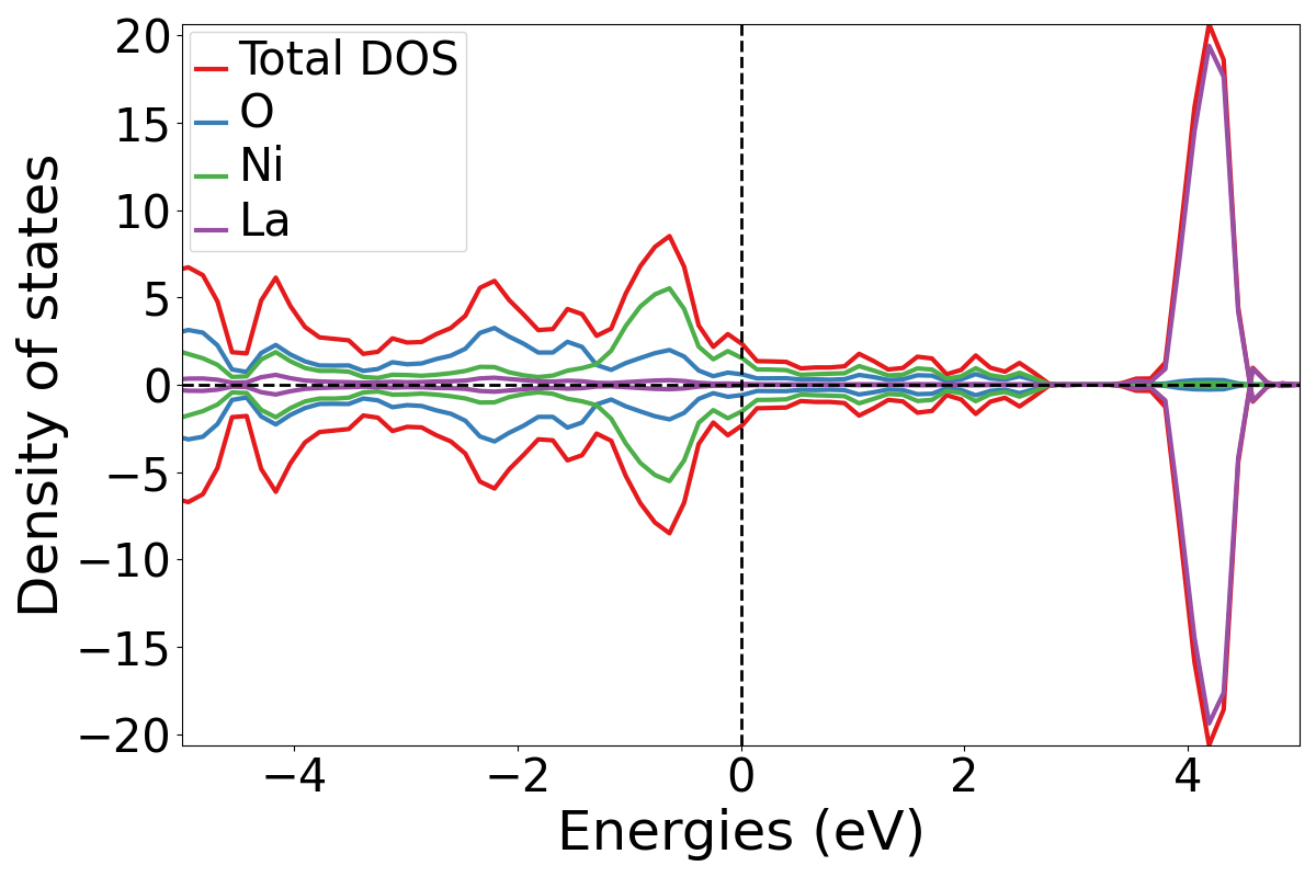
Atom Projected DOS

This plots the contribution to the DOS from each atom.

Run:

plotDOS.py atomic -show

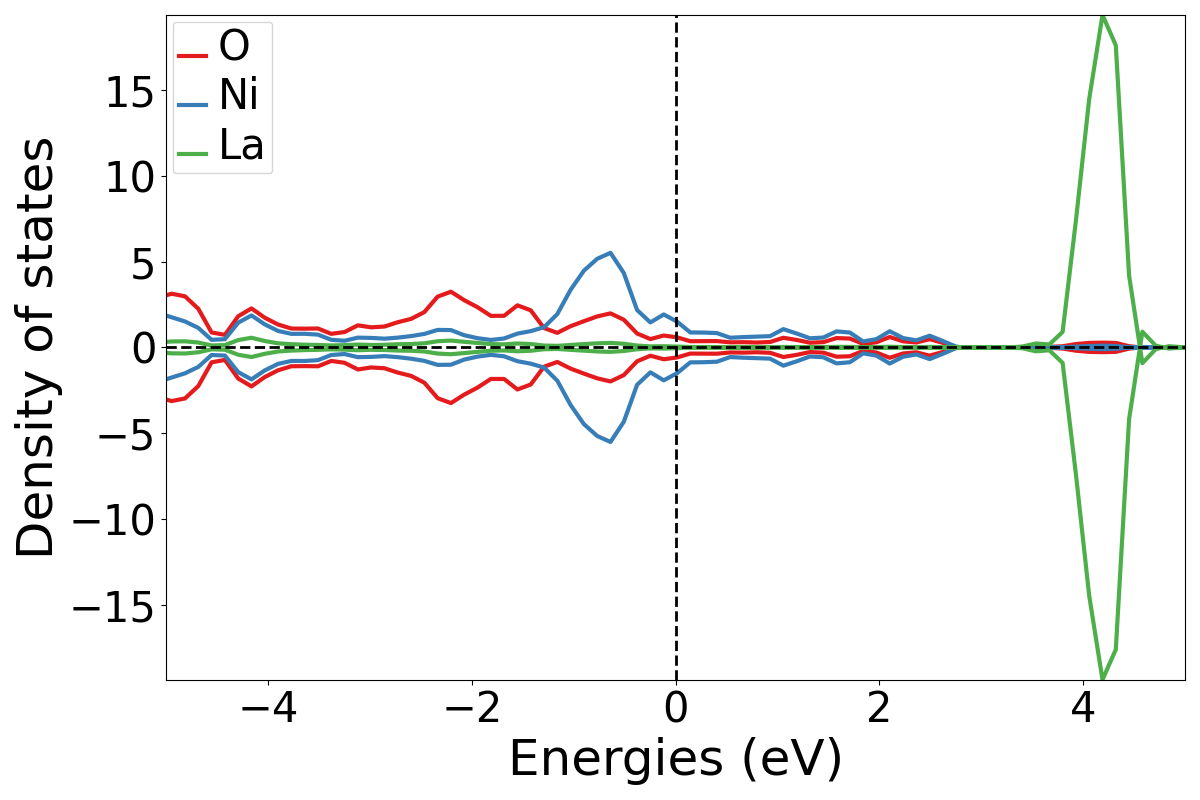
To see both the total and the atomic contributions on the same plot you may add the -total flag to the above command.

Orbital projected DOS

Next, let’s see how each orbital from the atoms contribute to the DOS. This enables us to observe how much each s, p, d or f orbital of a certain atom is present in the DOS. E.g. - Ni atom contribution

Run:

plotDOS.py orbital -atom Ni -show

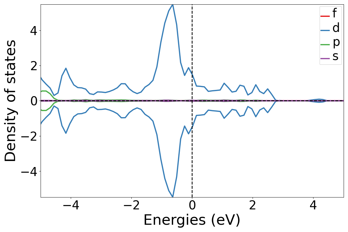
The -total flag works here as well if one wishes to see the total contribution for the orbital on the same plot.

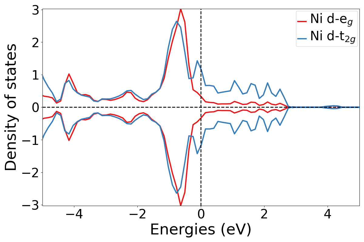
d-orbital projected DOS

In certain materials like strongly correlated systems where d orbitals play a vital role in conductivity and other properties, it is important to study the decomposed d-orbital projected DOS. i.e. the individual effects of the e\(_g\) and t\(_{2g}\) orbitals when the degeneracy of the d orbital is broken. Let’s consider the same example as above and investigate how the Ni d-orbitals behave.

Run:

plotDOS.py orbital_d -atom Ni -show

This would sum up the contribution from all the Ni atoms in the system. If you would like to customize the atoms, you could use a list. The indexes correspond to the order of the atoms in the POSCAR file.

E.g.- to sum the 3rd, 4th and 5th Ni atoms:

plotDOS.py orbital_d -l 3 4 5 -show

Imagine you have to perform such DOS calculations for a large set of calculations. You could use a simple bash command to achieve that. Assuming each of those calculations are in a seperate directory numbered as LaNiO3-1, LaNiO3-2 ….. LaNiO3-100, run:

for i in {1..100};do cd LaNiO3-$i && plotDOS.py orbital_d -atom Ni && cd ..;done

This would cd into each directory and run the script and repeat it for all the directories.

Well, that’s all for today. Please feel free to leave a comment if you have any questions or if you think I could incorporate any features into the script.

Be safe and stay home!

References

1. COrona VIrus Disease of 2019 ↩

2. http://electrons.wikidot.com/density-of-states ↩

3. https://www.vasp.at ↩

4. http://www.p4vasp.at ↩

5. https://github.com/materialsproject/pymatgen ↩